Abhinav's Tech Blog: Using Market Basket Analysis to add value to OLAP

Using Market Basket Analysis to add value to OLAP

Anyone who has an interest in data warehousing and/or business intelligence understands the concepts of dimensions and hierarchies, which are key parts of a multi-dimensional model. In most cases the structure of a hierarchy is driven the corporate business environment. For example, if we consider the common schema (SH) that is shipped with the 10g version of the database, the product dimension has one single hierarchy that is based on normal business levels: Categories, sub-categories and products.

Regular readers of this blog will might remember a posting from last year where I explained how you could use attribute importance to help determine the most important dimensions within a cube. This posting uses another data mining feature to help business users analyse product groupings.

Most people are aware of the concepts of a shopping cart from buying products online, and it can be extremely useful to track the contents of these baskets. Each basket can provide valuable insight into customer buying patterns and provide the opportunity to identify options for cross selling. Therefore, to analyse customer-purchasing behaviour we need to extract the following information

Which product combinations are bought?
When they are purchased? and in
What sequence?

Using the information extracted from this analysis new product dimensions (or product hierarchies) can be created to track these baskets and provide business users with the opportunity to create new types of reports:

What are my top 5 baskets?
What are my bottom 5 baskets?
Which baskets are the most profitable?
How are my top 5 baskets performing in my key target regions
How have my top 5 baskets been performing over the last 2 years
What is the revenue forecast for next year for my top 5 baskets

One of the many benefits of Oracle’s 10g database is packed with features and the trick to getting the maximum benefit from the investment in Enterprise Edition is to make these features work together.

In this case we can use an association rules algorithm, part of Oracle Data Mining, to create an alternative product hierarchy that can be used to provide additional insight into business operations.

The association rules (AR) algorithm predicts the probability of co-occurrence among sets of attribute values. The most well-know use case for AR is market basket analysis, which predicts items occurring together in a market checkout session. This type of hierarchy can be used to help identify cross sell opportunities and product bundle strategies as well as product placement within online and the more traditional bricks and mortar stores.

Creating a Market Basket Analysis

Creating the association rules model
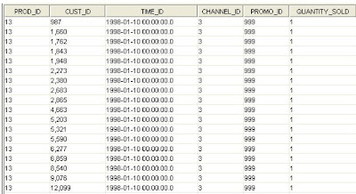
The sources for this example are the tables within the BI10g common schema. The SALES table contains point of sale data, which can be used as the main input to the market basket algorithm. To get started, you will need to have installed the Oracle Data Mining (ODM) Option (the default) during installation of the Oracle Database 10g. This ODM algorithm requires that the data be in this “transactional” format, with one item being represented in each row. This is an efficient representation, as any shopping basket will typically include several items from a possible hundreds or thousands of store items. The alternative, storing the data in a “single record per market basket”, would cause there to be hundreds to thousands of possible store items (attributes) with most of them being blank or null

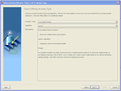
Launch Oracle Data Miner client (for download details see the links at the end of this posting). Select Build from the Activity pull-down menu to launch the activity, and select Association Rules from the Function Type pull-down menu. Click Next.

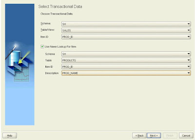
The transactions (market baskets) are contained in the SALES table; select PROD_ID as the identifier for the items purchased. However, the products are identified only by an item code; the names of the products are in the PRODUCTS table, so click the checkbox indicating that there is a Name Lookup table, and select the table, the item identifier (PROD_ID), and the column containing the item description (PROD_NAME). This will then create meaningful product descriptions in the results table that can then used to populate the description for the dimension.

Click Next to continue.

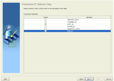
Two columns are required to identify a single market basket. Click the checkboxes for CUST_ID and TIME_ID, then click Next.

The final step is to enter a name for the activity and click Next. On the final page of the wizard, click Advanced Settings to see the parameters available for Association Rules. In this case the default settings can be used. However, there are a lot of parameters that can used to tune the model. For more information regarding these parameters please refer to the documentation for Oracle Data Mining 10g Release 2. This can be downloaded from OTN.

Click OK to return to the last page of the wizard and click Finish to run the activity. When the activity completes, click Result in the Build step to access the rules defined by the model.

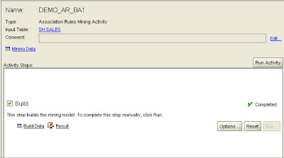
In this example, 115 rules were defined using the default parameter settings based on the transactions listed in the sales table

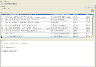
As well as the details of the products that comprise the rule two additional columns are provided: Confidence (%) and Support (%). The Support for the rule is the percentage of baskets containing the items in the rule. In the example, Support is the percentage of all baskets containing the three items mouse, keyboard and printer.
The Confidence for the rule is the percentage of baskets containing the item(s) in the antecedents that also contain the consequent. In the example, consider only baskets containing keyboard and mouse and calculate the percentage of those baskets that contain printers.

Saving the results
Finally, the results from the model can be published to a table. This table will then form the raw source for the new OLAP product dimension. Notice at this point there is no information relating to revenue, costs or quantity. All that information is already contained in the existing fact table that is used to feed the standard sales revenue, sales costs and sales quantity measures. All that needs to be done is to link the product bundles to the original fact table to extract the revenue, costs and quantity for each product within a bundle. The process for doing this will be explained later.

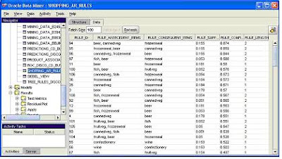
Designing the product dimension

The results from the algorithm table have to be transformed to provide a correctly formatted source for the dimension mapping. This requires the use of either OLAP DML (for those used to this powerful language) or PL/SQL. The aim is to create a new dimension table that confirms to the normal requirements for a source table. Therefore, a new top level has to be added to provide a total for “All Rules” and columns need to be populated for each of the attributes.

Each rule has to be broken down into its constituent parts:

The rule itself
The products that are part of the initial purchase
The products that are normally purchased in conjunction with the original items

From each rule the original product can be determined and referenced from the master Product Dimension.

This will allow us to track and analyze product bundles as part of the normal reporting process. Using the attributes associated with each rule, OLAP query steps can be created that further refine the analysis of product bundles by allowing business users to filter the results based on the value for % confidence associated with the rule.

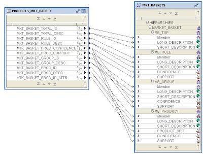
In this example the decision has been taken to create a separate dimension to hold the results from the algorithm. The dimension is based around a single hierarchy with the following levels:

Top level – All Baskets
Rule – Rule derived from the algorithm
Group – Contains the IF and THEN parts of the rule
Product – Base product

In an ideal world, this information would be used to create a custom aggregate for each rule within the Product Dimension. However, although Discoverer for OLAP now supports custom aggregates there is no public API to help with the creation process. Therefore, the only way forward with this is to use a separate dimension to hold the rules.

This structure is outlined below with the associated attributes of:

Long description
Short description
Source product
Confidence %
Support %

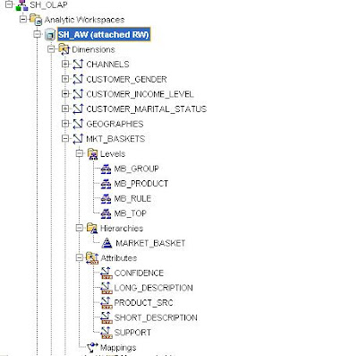
The finished mapping looks like this:

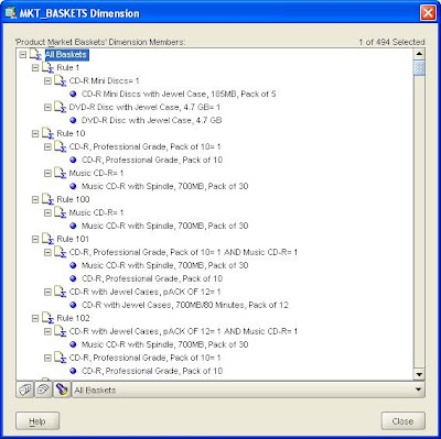
Once the dimension has been maintained you can use the Dimension Viewer to check the results.

Designing the cube

The next requirement is to create a new source table that can be used in the mapping for the cube. Again some coding is required to create this new fact table. The code needs to extract the source products from each rule and identify the associated costs, revenue and quantity from the original fact table. This will then be moved to a new fact table to make mapping and loading data much easier to manager.

The new fact table looks like this:

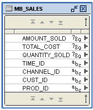
When the cube is aggregated it will be possible to view the total revenue, total cost, total quantity, margin etc derived from the various products that are part of the rule.

A new cube called “MB” is created and the all the usual dimensions except in this case the new market basket dimension replaces PRODUCT dimension. The definition of the cube follows the same pattern as the other cubes in the sample schema.

In this case the figure for “All Baskets” which is the top level of the new market basket dimension is largely irrelevant. The reason for this is because the same product can appear in multiple rules, therefore, the value for total revenue, or total cost or total quantity is based on double counting of values. So this top value has to be treated with caution.

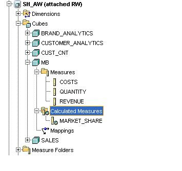Now it is possible to create all the usual calculated measures for each of the base measures associated with a product bundle (revenue, costs, quantity, and margin) , such as those linked to the other cubes that are part of the common schema sample. For example:

12 month moving average
6 month moving average
Percent growth prior period
Percent growth prior year
Forecast
% Share of total revenue
% Share of total cost
% Share of total quantity

For the share calculations the formula needs to reach back to the original sales revenue cube that is dimensioned by the original product dimension. For this an OLAP DML formula is used which looks like this:

MB_REVENUE/SALES_REVENUE(PRODUCTS '1')*100

All these new measures can finally be added to a new measure folder called Market Basket Analysis and everything is ready for access by Discoverer OLAP, BI Beans and/or Spreadsheet Addin.

So what does this provide? With this cube it will now be possible to answer the following types of questions:

What are my top 5 baskets?
What are my bottom 5 baskets?
Which baskets are the most profitable?
How are my top 5 baskets performing in my key target regions
How have my top 5 baskets been performing over the last 2 years
What is the revenue forecast for next year for my top 5 baskets

Viewing the Results in Excel

Using Spreadsheet Addin it is now possible to connect to the updated schema. Launching the query builder shows the new dimension (Product Market Baskets) and the associated new measures for the market basket analysis

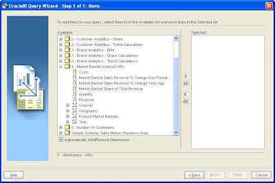
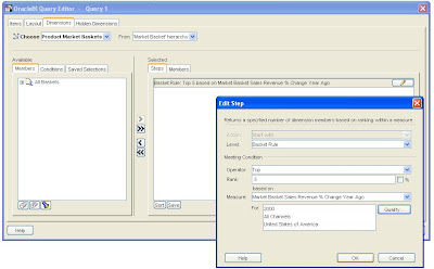
With this new dimension it is now possible to analyze the performance of each basket in the context of % growth prior period, % growth prior year etc. An obvious report to create is to show the performance of the top 5 baskets based on % growth prior year for year 2000, within the USA across All Channels.

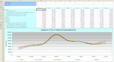
The results from this query can be plotted on a line graph to show the revenue trend over the last 8 quarters as shown below.

Abhinav's Tech Blog

Pages

Thursday, February 15, 2007

Using Market Basket Analysis to add value to OLAP